DEmoClassi

DEmoClassi stands for Demographic (age, gender, race) and Emotions (happy, sad, angry, ...) Classification from face images, using deep learning.

Project maintained by AlkaSaliss Hosted on GitHub Pages — Theme by mattgraham

An attempt to predict emotion, age, gender and race from face images using Pytorch

During my internship, when I started reading papers in NLP implementing neural network architectures with dynamic computation graphs, I felt the need to switch to a framework other than Tensorflow. This is how I discovered Pytorch and was really attracted by its simplicity given my Python background.

After doing all the tutorial from the official pytorch website, I thought it might be interesting for me to try and implement a project end-to-end using pytorch so that I can ensure myself I really understood how Pytorch works under the hood. I ended up doing this funny project I named DEmoClassi which stands for : Demographic (age, gender, race) and Emotion Classification. It consists simply of predicting the age, gender, race and facial expression of a person from his/her face image.

In this post, I’ll try to explain how I dealt with this task using pytorch and pytorch-ignite (a high-level wrapper of pytroch).

The post will consist of the following :

Presenting the datasets I used
Models training
Performance evaluation
and finally model deployment using opencv ot make predicitions in real-time

1. Prepare the environment on google colab

Training deep learning models requires sometimes GPU to train faster and thus to be able to experiment with various architectures. Fortunately enough, Google Colab provides jupyter notebooks attached to backends with GPU support for free. For more information on how to get started with google colab, this link, this one and also this one are good places to start with.

However, I used to program my functions during my daily commute and don’t necessarily have access to internet connection at this time. So for productivity reasons I decided to gather all the utility functions I develop during my commute in a pip installable package so that when I come home I can just do
pip install my-awesome-package on google colab and start model training. That’s how I created my first package called democlassi which is just a collection of my utility functions/classes to easy data processing, model training and evaluation.

So to start let’s install the so called democlassi package :

pip install --upgrade democlassi

That’s it, now I have access to my functions and can move to the next step : get the data in !

Let’s also import all the necessary modules we’ll need later.

import torch
import torchvision.transforms as transforms

from vision_utils.custom_torch_utils import load_model
from vision_utils.custom_architectures import SepConvModelMT, SepConvModel, initialize_model

from emotion_detection.evaluate import evaluate_model as eval_fer
from emotion_detection.fer_data_utils import get_fer_dataloader
from emotion_detection.train import run_fer

from multitask_rag.train import run_utk
from multitask_rag.utk_data_utils import get_utk_dataloader
from multitask_rag.evaluate import evaluate_model as eval_utk
from multitask_rag.utk_data_utils import display_examples_utk

import pandas as pd
import glob
import os
import random

from google.colab import drive

2. The datasets

First of all, let’s connect our google drive to the currently running google colab notebook by running the following :

drive.mount('gdrive')

This command will prompt you with a token that you can click and it will redirect you to your google account so that you can authenticate yourself.

I like connecting to my google drive because it allows me to save periodically my model checkpoints during training, which is quite useful in case you lose your connection or an error happens during training.

Now my google drive is mounted at '/content/gdrive/My Drive' and if I execute the following command I can see the list of my files and folders

!ls '/content/gdrive/My Drive' 

I used two different datasets for the tasks at hand :

2.1. Fer2013 dataset

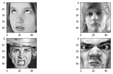
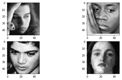
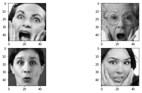
Fer2013 is a kaggle dataset which consists of a set of 48x48 grayscale images representing the following facial expressions : * 0 : Angry * 1 : Disgust * 2 : Fear * 3 : Happy * 4 : Sad * 5 : Surprise * 6 : Neutral

One can download the data here and extract the csv containing training, validation and test sets. Let’s visualize some sample images form the dataset.

# Reading the data
path_fer = './fer2013.csv'  # or whatever the path to the downloaded data is
df_fer2013 = pd.read_csv(path_fer)

display_examples_fer(df, 0)

Sample images for class : Angry

png

display_examples_fer(df, 1)

Sample images for class : Disgust

png

display_examples_fer(df, 2)

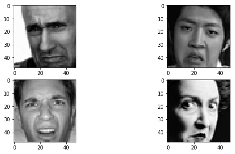
Sample images for class : Fear

png

display_examples_fer(df, 3)

Sample images for class : Happy

png

display_examples_fer(df, 4)

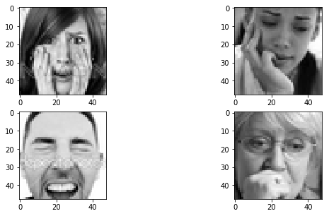
Sample images for class : Sad

png

display_examples_fer(df, 5)

Sample images for class : Surprise

png

display_examples_fer(df, 6)

Sample images for class : Neutral

png

I don’t know if it is the case for everyone else who worked on this dataset, but sometimes I find it quite difficult to visually distinguish between some classes, especially between disgust, Angry and fear, or between sad and neutral, etc. This is understandable given that even in real life it’s much more easier to tell if a person face expression is positive or negative, than telling the expression in lower granularity (fear, sad, happy, angry, …).

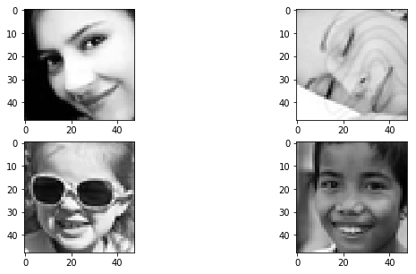
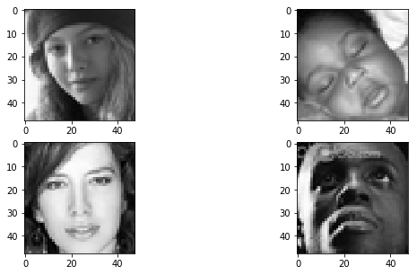
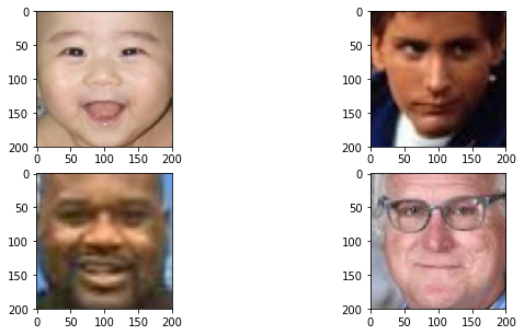
2.2. UTK face dataset

This is a dataset of cropped face images for the task of predicting the age, gender and race of a person. One can download the data here and extract the directory containing the images

The labels for this dataset consists of :

Age : is an number between 0 and 101 (representing the age of the person)
Gender :
- 0 : Male
- 1 : Female
Race :
- 0 : White
- 1 : Black
- 2 : Asian
- 3 : Indian
- 4 : Other

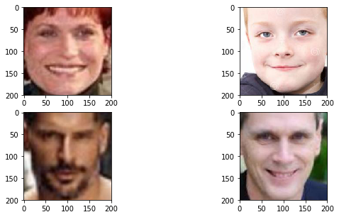
Let’s visualize some sample images from the utk face dataset :

path_utk = './UTKFace/'  # or whatever the path to the downloaded and extracted utk face images

display_examples_utk(path_utk, 'gender', 0)

Sample images for gender : Male

png

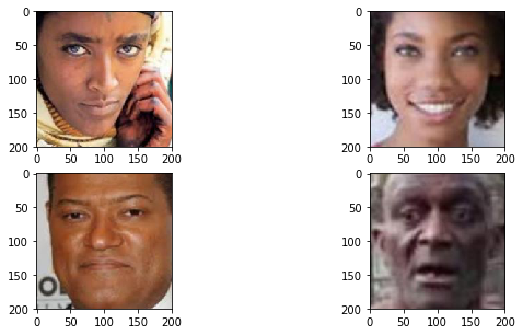
display_examples_utk(path_utk, 'race', 0)

Sample images for race : White

png

display_examples_utk(path_utk, 'race', 1)

Sample images for race : Black

png

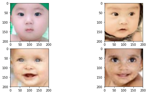
display_examples_utk(path_utk, 'age', 1)

Sample images for age : 1

png

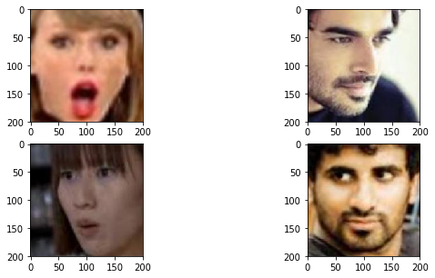
display_examples_utk(path_utk, 'age', 25)

Sample images for age : 25

png

3. Training

Now that we have the data ready, let’s move to the funniest part : model training! As I have two separate datasets (Fer2013 for emotion detection and UTKFace for gender-race-age prediction) we’ll have to train two separate models. For each of the two tasks I tested 3 different architectures :

A CNN based on Depthwise Separable Convolution
Finetuning a pretrained Resnet50
Finetuning a pretrained VGG19

3.1 Training emotion detector

a. Depthwise Separable Convolution model

First we need to create DataLoader objects which are handy Pytorch objects for yielding batches of data during training. Basically, what the following code does is :

read the csv file and convert the raw pixels into numpy arrays
Apply some pre-processing operations :
- Histogram equalization (see here for more information)
- Add a channel dimension so that the image becomes 48x48x1 instead of 48x48
- Convert the numpy array to a pytorch tensor

DATA_DIR = "./fer2013.csv" # path to the csv file
BATCH_SIZE = 256 # size of batches 
train_flag = 'Training' # in the csv file there's a column `Usage` which represents the usage of the data : train or validation or test
val_flag = 'PublicTest'

# The transformations to apply
data_transforms = transforms.Compose([
    HistEq(), # Apply histogram equalization
    AddChannel(), # Add channel dimension to be able to apply convolutions
    transforms.ToTensor()
])

train_dataloader = get_fer_dataloader(BATCH_SIZE, DATA_DIR, train_flag, data_transforms=data_transforms)
validation_dataloader = get_fer_dataloader(BATCH_SIZE, DATA_DIR, val_flag, data_transforms=data_transforms)

my_data_loaders = {
    'train': train_dataloader,
    'valid': validation_dataloader
}

Create a model and an optimizer, and start training

SepConvModel is a custom implementation of Separable convolution layers in Pytorch.

my_model = SepConvModel()  # 
my_optimizer = torch.optim.Adam(my_model.parameters(), lr=1e-3)

backup_path is the path to a folder in my google drive where I would like to copy model checkpoints to, during training a kind of periodic backup in case I lose connection during training.

backup_path = '/content/gdrive/My Drive/Face_detection/checkpoints/sepconv_adam_histeq'
os.makedirs(backup_path, exist_ok=True)  # create the directory if it doesn't exist
checkpoint = '/content/checkpoints/sep_conv'  # folder where to save checkpoints during training

Now for the model training function some parameters are quite intuitive, but here are some that aren’t:

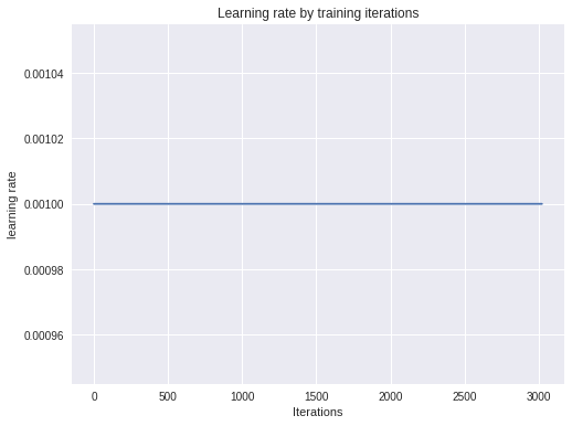
log_interval is the number of iterations before printing training loss
dirname is the directory where to save model checkpoints
n_saved : number of best model checkpoints to save, e.g. if 3 then the 3 best models obtained during training will be saved
filename_prefix : name of the file under which to save model checkpoints, e.g. my_sep_conv_model
launch_tensorboard : if True creates tensorboard summaries
log_dir path where to save tensorboard logs if launch_tensorboard is set to True
patience=50 is the number of epochs to wait for before stopping training if no improvement is observed

For additional details on other parameters one can check the function run_fer docstring.

run_fer(model=my_model, optimizer=my_optimizer, epochs=300, log_interval=1, dataloaders=my_data_loaders,
        dirname=checkpoint,
        n_saved=1,
        log_dir=None,
        launch_tensorboard=False, patience=50,
        resume_model=None, resume_optimizer=None, backup_step=5, backup_path=backup_path,
        n_epochs_freeze=0, n_cycle=None)

Number of trainable parameters : 706,001
Number of non-trainable parameters : 0

ITERATION - loss: 0.635: 100%|██████████| 57/57 [01:01<00:00,  2.59it/s]

Training Results - Epoch: 1  Avg accuracy: 0.661 Avg loss: 0.918

ITERATION - loss: 0.635: 100%|██████████| 57/57 [01:05<00:00,  2.59it/s]

Validation Results - Epoch: 1  Avg accuracy: 0.570 Avg loss: 1.187

ITERATION - loss: 0.548: 100%|██████████| 57/57 [02:07<00:00,  2.59it/s]

Training Results - Epoch: 2  Avg accuracy: 0.675 Avg loss: 0.877

ITERATION - loss: 0.548: 100%|██████████| 57/57 [02:12<00:00,  2.59it/s]

Validation Results - Epoch: 2  Avg accuracy: 0.572 Avg loss: 1.175

ITERATION - loss: 0.532: 100%|██████████| 57/57 [03:13<00:00,  2.58it/s]

Training Results - Epoch: 3  Avg accuracy: 0.668 Avg loss: 0.890

ITERATION - loss: 0.532: 100%|██████████| 57/57 [03:18<00:00,  2.58it/s]

Validation Results - Epoch: 3  Avg accuracy: 0.572 Avg loss: 1.189

              .......
              
ITERATION - loss: 0.108: 100%|██████████| 57/57 [58:25<00:00,  2.56it/s]

Training Results - Epoch: 53  Avg accuracy: 0.926 Avg loss: 0.222

ITERATION - loss: 0.108: 100%|██████████| 57/57 [58:30<00:00,  2.56it/s]

Validation Results - Epoch: 53  Avg accuracy: 0.578 Avg loss: 1.626

png

The execution took 0.0 hours | 58.0 minutes | 50.3 seconds!

3.4. Resnet-50

Next we train a resnet model.

Let’s define the data transformations as previously :

# The transformations to 
data_transforms = transforms.Compose([
    HistEq(), # Apply histogram equalization
    ToRGB(), 
    transforms.ToTensor()
])

Here we added an extra preprocessing operation ToRGB() which takes a 1-channel (H x W x 1) array and convert it into 3-channel (H x W x 3) array by just repeating the array 3 times along the channel axis.

And create training and validation DataLoaders as previously :

my_data_loaders = {
    'train': get_fer_dataloader(BATCH_SIZE, DATA_DIR, train_flag, data_transforms=data_transforms),
    'valid': get_fer_dataloader(BATCH_SIZE, DATA_DIR, val_flag, data_transforms=data_transforms)
}

Create a model and an optimizer, and start training

backup_path = '/content/gdrive/My Drive/Face_detection/checkpoints/resnet_adam_histeq'
os.makedirs(backup_path, exist_ok=True)

The initialize_model() function creates a pretrained model specified by the argument model_name which can take values such as ‘resnet’, ‘vgg’, ‘alexnet’, ‘inception’, … and returns the model with the input size. If the argument feature_extract is set to True the pretrained layers are frozen.

my_model, _ = initialize_model(model_name='resnet', feature_extract=True, num_classes=7,
                               task='fer2013', use_pretrained=True)
# The optimizer must only track the parameters that are trainable (thus excluding frozen ones)
my_optimizer = torch.optim.Adam(filter(lambda p: p.requires_grad, my_model.parameters()), lr=1e-3) 

Downloading: "https://download.pytorch.org/models/resnet50-19c8e357.pth" to /root/.torch/models/resnet50-19c8e357.pth
102502400it [00:01, 85233773.18it/s]

In addition, the parameter n_epochs_freeze for the function run_fer controls the number of epochs before unfreezing the frozen layers for finetuning.

run_fer(model=my_model, optimizer=my_optimizer, epochs=200, log_interval=1, dataloaders=my_data_loaders,
        dirname='/content/checkpoints/resnet_adam_histeq', filename_prefix='resnet',
        n_saved=1,
        log_dir=None,
        launch_tensorboard=False, patience=75, val_monitor='acc',
        resume_model=None, resume_optimizer=None, backup_step=5, backup_path=None,
        n_epochs_freeze=10, n_cycle=None)

Number of trainable parameters : 14,343
Number of non-trainable parameters : 23,508,032

ITERATION - loss: 1.560: 100%|██████████| 113/113 [01:04<00:00,  6.67it/s]

Training Results - Epoch: 1  Avg accuracy: 0.353 Avg loss: 1.660

ITERATION - loss: 1.560: 100%|██████████| 113/113 [01:09<00:00,  6.67it/s]

Validation Results - Epoch: 1  Avg accuracy: 0.318 Avg loss: 1.720

ITERATION - loss: 1.348: 100%|██████████| 113/113 [02:13<00:00,  7.37it/s]

Training Results - Epoch: 2  Avg accuracy: 0.377 Avg loss: 1.616

ITERATION - loss: 1.348: 100%|██████████| 113/113 [02:18<00:00,  7.37it/s]

Validation Results - Epoch: 2  Avg accuracy: 0.334 Avg loss: 1.696

                               ...

Validation Results - Epoch: 9  Avg accuracy: 0.344 Avg loss: 1.680
****Unfreezing frozen layers ... ***
Number of trainable parameters : 23,522,375
Number of non-trainable parameters : 0 ;

ITERATION - loss: 1.017: 100%|██████████| 113/113 [12:46<00:00,  1.36it/s]

Training Results - Epoch: 10  Avg accuracy: 0.528 Avg loss: 1.263

ITERATION - loss: 1.017: 100%|██████████| 113/113 [12:51<00:00,  1.36it/s]

Validation Results - Epoch: 10  Avg accuracy: 0.492 Avg loss: 1.339

                            ....
                            
ITERATION - loss: 0.000: 100%|██████████| 113/113 [5:05:59<00:00,  1.37it/s]

Training Results - Epoch: 130  Avg accuracy: 0.998 Avg loss: 0.027

Validation Results - Epoch: 130  Avg accuracy: 0.607 Avg loss: 3.489

png

The execution took 5.0 hours | 6.0 minutes | 10.1 seconds!

3.5 VGG-19

The routine is the same as previously :

creates data loaders
instantiate a model and optimizer
and start training

# The transformations to 
data_transforms = transforms.Compose([
    HistEq(),
    ToRGB(), 
    transforms.ToTensor()
])

my_data_loaders = {
    'train': get_fer_dataloader(256, DATA_DIR, train_flag, data_transforms=data_transforms),
    'valid': get_fer_dataloader(512, DATA_DIR, val_flag, data_transforms=data_transforms)
}


my_model, _ = initialize_model(mosdel_name='vgg', feature_extract=True, num_classes=7,
                               task='fer2013', use_pretrained=True)
my_optimizer = torch.optim.Adam(filter(lambda p: p.requires_grad, my_model.parameters()), lr=1e-3)

Downloading: "https://download.pytorch.org/models/vgg19_bn-c79401a0.pth" to /root/.torch/models/vgg19_bn-c79401a0.pth
574769405it [00:06, 86558268.30it/s]

backup_path = '/content/gdrive/My Drive/Face_detection/checkpoints/vgg_adam_histeq'

os.makedirs(backup_path, exist_ok=True)

run_fer(model=my_model, optimizer=my_optimizer, epochs=300, log_interval=1, dataloaders=my_data_loaders,
        dirname='/content/checkpoints/vgg_adam_histeq', filename_prefix='vgg',
        n_saved=1,
        log_dir=None,
        launch_tensorboard=False, patience=100, val_monitor='acc',
        resume_model=None, resume_optimizer=None, backup_step=5, backup_path=backup_path,
        n_epochs_freeze=20, n_cycle=None)

ITERATION - loss: 0.000:   0%|          | 0/113 [00:00<?, ?it/s]

Number of trainable parameters : 28,679
Number of non-trainable parameters : 139,581,248

ITERATION - loss: 1.809: 100%|██████████| 113/113 [01:16<00:00,  3.42it/s]

Training Results - Epoch: 1  Avg accuracy: 0.338 Avg loss: 1.655

ITERATION - loss: 1.809: 100%|██████████| 113/113 [01:24<00:00,  3.42it/s]

Validation Results - Epoch: 1  Avg accuracy: 0.319 Avg loss: 1.704

ITERATION - loss: 1.412: 100%|██████████| 113/113 [02:42<00:00,  3.40it/s]

Training Results - Epoch: 2  Avg accuracy: 0.353 Avg loss: 1.627

ITERATION - loss: 1.412: 100%|██████████| 113/113 [02:50<00:00,  3.40it/s]

Validation Results - Epoch: 2  Avg accuracy: 0.320 Avg loss: 1.698

ITERATION - loss: 1.370: 100%|██████████| 113/113 [04:08<00:00,  3.40it/s]

                    .....
                    
Training Results - Epoch: 19  Avg accuracy: 0.388 Avg loss: 1.560

ITERATION - loss: 1.166: 100%|██████████| 113/113 [26:57<00:00,  3.37it/s]

Validation Results - Epoch: 19  Avg accuracy: 0.336 Avg loss: 1.674

****Unfreezing frozen layers ... ***
Number of trainable parameters : 139,609,927
Number of non-trainable parameters : 0

ITERATION - loss: 1.161: 100%|██████████| 113/113 [30:10<00:00,  1.06s/it]

Training Results - Epoch: 20  Avg accuracy: 0.517 Avg loss: 1.243

ITERATION - loss: 1.161: 100%|██████████| 113/113 [30:18<00:00,  1.06s/it]

Validation Results - Epoch: 20  Avg accuracy: 0.492 Avg loss: 1.296

                        ....
                        
Training Results - Epoch: 126  Avg accuracy: 0.987 Avg loss: 0.041

ITERATION - loss: 0.000: 100%|██████████| 113/113 [6:30:33<00:00,  1.06s/it]

Validation Results - Epoch: 126  Avg accuracy: 0.620 Avg loss: 4.564

And that’s it for the training of the 3 models : separable convolution, Resnet50 and VGG19. The training procedure for the second task (age, gender and race prediction) is quite similar to that presented here:

prepare the data and apply eventually some transformations
create models (separable conv, or pretrained vg, resnet …)
and train Check this notebook for the entire training process for the second task.

4. Evaluation

Now that we have some trained models, we can assess their performance on the test which wasn’t used neither for training nor for validation.

We define the paths to the saved model checkpoints :

path_fer_sepconv = '/content/gdrive/My Drive/Face_detection/checkpoints/sepconv_adam_histeq/sepconv_model_55_val_loss=1.175765.pth'
path_fer_resnet = '/content/gdrive/My Drive/Face_detection/checkpoints/resnet_adam_histeq/resnet_model_109_val_accuracy=0.6227361.pth'
path_fer_vgg = '/content/gdrive/My Drive/Face_detection/checkpoints/vgg_adam_histeq/vgg_model_173_val_accuracy=0.6447478.pth'

The saved models are not actually the models themselves, but rather their weights, which in pytorch terms are called state_dict. So in order to retrieve a trained model, we need to recreate the model instance, then load its weight. Let’s define our three models instances : a depthwise separable-convolution, a resnet-50 and a vgg-19 :

model_fer_sepconv = SepConvModel()
model_fer_resnet, _ = initialize_model('resnet', feature_extract=False, use_pretrained=False)
model_fer_vgg, _ = initialize_model('vgg', feature_extract=False, use_pretrained=False)

And next we define our data transformation operations, and create a the dataloaders

data_transforms_fer = transforms.Compose([
    HistEq(),
    AddChannel(),
    transforms.ToTensor()
])

# data transforms for the pretrained models
data_transforms_fer_tl = transforms.Compose([
    HistEq(),
    ToRGB(),
    transforms.ToTensor()
])

dataloader_fer = get_fer_dataloader(256, path_fer, 'PrivateTest', data_transforms=data_transforms_fer)

dataloader_fer_tl = get_fer_dataloader(256, path_fer, 'PrivateTest', data_transforms=data_transforms_fer_tl)

4.1 Evaluate Separable conv model

Load the saved weights into the model’s instance :

model_fer_sepconv.load_state_dict(torch.load(path_fer_sepconv))

and evaluate :

evaluate_fer(model_fer_sepconv, dataloader_fer,
                   title='Confusion matrix - Test set')

100%|██████████| 15/15 [00:03<00:00,  4.57it/s]


              precision    recall  f1-score   support

       Angry       0.51      0.41      0.45       491
     Disgust       0.00      0.00      0.00        55
        Fear       0.44      0.15      0.23       528
       Happy       0.70      0.87      0.78       879
         Sad       0.42      0.39      0.41       594
    Surprise       0.65      0.74      0.69       416
     Neutral       0.47      0.68      0.56       626

   micro avg       0.56      0.56      0.56      3589
   macro avg       0.46      0.46      0.45      3589
weighted avg       0.54      0.56      0.53      3589

png

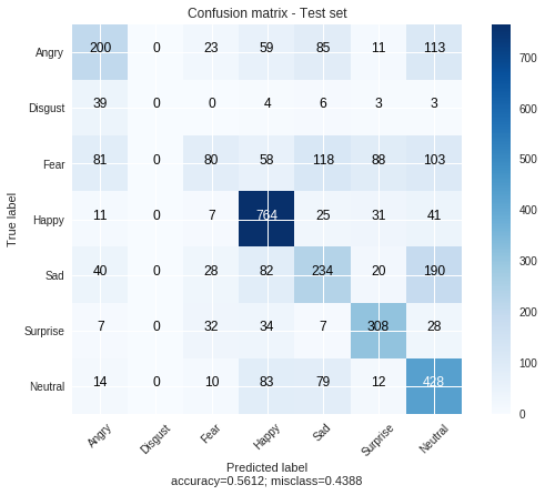
The execution took 0.0 hours | 0.0 minutes | 4.1 seconds!

4.2 Evaluate Resnet models

model_fer_resnet.load_state_dict(torch.load(path_fer_resnet))

evaluate_fer(model_fer_resnet, dataloader_fer_mt,
                   title='Confusion matrix - Test set')

100%|██████████| 15/15 [00:04<00:00,  3.33it/s]


              precision    recall  f1-score   support

       Angry       0.50      0.52      0.51       491
     Disgust       0.72      0.62      0.67        55
        Fear       0.54      0.46      0.49       528
       Happy       0.79      0.86      0.82       879
         Sad       0.49      0.54      0.51       594
    Surprise       0.77      0.74      0.75       416
     Neutral       0.60      0.56      0.58       626

   micro avg       0.63      0.63      0.63      3589
   macro avg       0.63      0.61      0.62      3589
weighted avg       0.63      0.63      0.63      3589

png

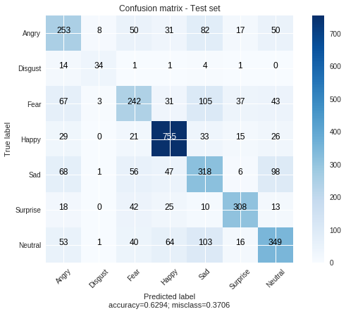
The execution took 0.0 hours | 0.0 minutes | 5.3 seconds!

4.3 Evaluate VGG models

model_fer_vgg.load_state_dict(torch.load(path_fer_vgg))

evaluate_fer(model_fer_vgg, dataloader_fer_mt,
                   title='Confusion matrix - Test set')

100%|██████████| 15/15 [00:06<00:00,  2.15it/s]


              precision    recall  f1-score   support

       Angry       0.60      0.54      0.57       491
     Disgust       0.68      0.58      0.63        55
        Fear       0.51      0.47      0.49       528
       Happy       0.87      0.82      0.85       879
         Sad       0.51      0.48      0.50       594
    Surprise       0.74      0.78      0.76       416
     Neutral       0.55      0.70      0.62       626

   micro avg       0.64      0.64      0.64      3589
   macro avg       0.64      0.62      0.63      3589
weighted avg       0.65      0.64      0.64      3589

png

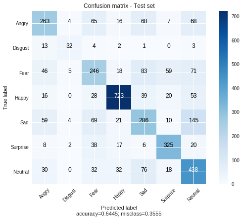
The execution took 0.0 hours | 0.0 minutes | 7.9 seconds!

That’s it for the evaluation of the emotion detection task. We can see that the best model here is the VGG19 with about 65% of accuracy. For the evaluation of the second task, check this notebook.

5. Real time prediction using opencv

Once we have trained and select the best model from evaluation on test set, we can test its performance in real time using opencv to and our webcam to capture images in streaming fashion. However this is done locally as I didn’t find a way doing streaming images processing with opencv on Google colab. Install opencv with pip install opencv-python from your terminal

The pretrained models can be downloaded from google drive :

Emotion detection :
- Separable conv : link
- Resnet : link
- VGG : link
Age, gender and race prediction :
- Separable conv : link
- Resnet : link
- VGG : link

Let’s say for instance we want to use the VGG model for emotion detection, and resnet model for age-gender-race prediction, we can execute deploy them using the following command :

python -m vision_utils.cv2_deploy \
        --emotion_model_weight path_to_my_emotion_model \
        --demogr_model_weight path_to_age_gender_race_prediction_model \
        --type_emotion_model vgg \
        --type_demog_model resnet \
        --source stream

path_to_my_emotion_model and path_to_age_gender_race_prediction_model should be replace with the path to the pretrained models resp. The command should load the models and start the webcam for live prediction. Note : the loading could take few seconds depending on the machine’s capacity and the model chosen, e.g. the VGG model’s weight are quite big in terms of size so it may be slower than using the separable conv model.

For more information on the possible arguments for teh detection using opencv you can use the help option to print all arguments :

python -m vision_utils.cv2_deploy -h

Final words

That’s it for this project. So where to go from here ?

Test other architectures : densenet, inception, …
Test with various different optimizers, regularization techniques, learing rates …
Put your idea here

This the first deeplearning project I carried out end-to-end, so I’ll be happy to welcome all your suggestions regarding what I could have done better.

Project Github link